WGT makes Wheeler graph research practical by packaging generators, a recognizer, and visualizations for the edge-labeled graphs that can be indexed like a Burrows-Wheeler Transform. It explains why recognition is computationally difficult, how Wheelie combines a renaming heuristic with permutation and SMT solvers, and how visualization helps inspect graph-index structures.
Modern genomics is moving away from a single linear reference toward the pangenome — many genomes represented together, usually as a graph, so that all the variation between individuals is in the picture rather than flattened into one consensus. But a pangenome is only useful if you can search it: given a sequencing read, you need to find where it matches, and you need that to be fast even when the graph encodes thousands of genomes.
For a single linear genome we have a beautiful answer to this: the Burrows-Wheeler Transform (BWT; Burrows and Wheeler, 1994) and the FM-index (Ferragina and Manzini, 2005), which let you index a genome once and then answer queries in time that scales with the query, not the genome. The natural question for pangenomes is whether the same trick works on a graph. Remarkably, for a special class of graphs, it does. Those are Wheeler graphs (Gagie et al., 2017), and they’re the elegant structure quietly underpinning graph-based pangenome indexes.
WGT, the Wheeler Graph Toolkit (Chao et al., 2023), is the software we built to make Wheeler graphs something you can actually work with.
What’s a Wheeler graph — and why it was hard to use
A Wheeler graph is a directed, edge-labeled graph whose nodes can be put in a special order — one that generalizes the sorting at the heart of the BWT. That order supports compact BWT-like indexes and efficient path queries on the graph. This connection is why Wheeler graphs form part of the theoretical basis for pangenome tools such as vg (Garrison et al., 2018).
More precisely, every zero-indegree node (a node with no incoming edges) must appear before every other node. Then consider two edges, from u to v with label a and from u′ to v′ with label a′. If a comes before a′, then v must come before v′. If the labels are equal and u comes before u′, then v cannot come after v′. The animation below turns those conditions into a visible ordering rule.
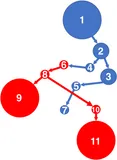
The walkthrough uses the eight-node graph shown later in Figure 1. It preserves all of that graph’s nodes and edges, but adapts the labels to the full DNA alphabet: the two edges entering S8 are shown as T, giving the ordered classes A, C, G, and T.
See why this DNA graph is Wheeler
Figure 1, adapted
The Figure 1 topology shares nodes and edges among many paths. Each directed edge contributes A, C, G, or T to the DNA sequence spelled along a path.
1Read sequence paths through one DNA graph
2Put the zero-indegree node first
3Form destination blocks in DNA order
4Preserve source order within each base
5Read the final Wheeler order
Eight nodes and thirteen DNA-labeled edges share one graph; S2 is the only zero-indegree node.
1 / 5
zero indegreevalid order
Here’s the catch that motivated us. Given some graph you’ve built, is it a Wheeler graph — does a valid ordering exist? That recognition problem is NP-complete in general, and hard even to approximate (Gibney and Thankachan, 2019). A theoretical algorithm had been proposed, but there was no working implementation — no way to actually feed it a graph and get an answer. And beyond recognition, there were no practical tools to visualize a Wheeler graph, or to generate example graphs to test ideas on. The concept was foundational, and yet almost untouchable in practice.
WGT began as the final project for Ben Langmead’s Computational Genomics: Sequences class at Johns Hopkins, in the fall of 2021 — an assignment that turned out to ask a question with no working answer. I kept building it the next spring in Ben’s Sketching and Indexing for Sequences class, a fitting home: its subject is the succinct, compressed indexes that let you search inside long, repetitive text — the lineage that Wheeler graphs carry from a string to a graph. From there it grew into a lab project with Pei-Wei Chen and Sanjit Seshia at UC Berkeley, whose formal-methods expertise led us to use satisfiability modulo theories (SMT) for the unresolved ordering constraints. Our goal was simple to state: make Wheeler graphs practical to generate, check, and see.
What WGT is
WGT is an open-source suite with three parts, shown end to end below.
Figure 1. The Wheeler Graph Toolkit, end to end. A generator produces a graph (Wheeler or not); the recognizer, Wheelie, decides whether the graph is a Wheeler graph and, if so, finds a valid node ordering — first applying a renaming heuristic, then handing the remaining work to a permutation solver or an SMT solver; and a visualizer draws the result. The interactive walkthroughs retain this graph’s topology while adapting its three abstract label classes to A, C, G, and T.
The three parts are:
Generators that produce graphs to work with — De Bruijn graphs (which encode overlapping fixed-length subsequences) and tries built from sequences, reverse-deterministic graphs built from multiple sequence alignments, and random graphs (including tunable “d-NFA” graphs) where you control the number of nodes, the edges, the alphabet size, and the branching. This gives you a steady supply of both Wheeler and non-Wheeler graphs to test on.
A recognizer, the core of the toolkit, called Wheelie.
A visualizer that draws a graph in a “two replicas” bipartite layout — the ordered nodes appear in two rows, with edges leaving one row and arriving in the other — which makes the otherwise-abstract Wheeler ordering something you can actually look at.
To make that concrete, here is WGT applied to a real gene: take the human gene STAU2 and its orthologs, build a De Bruijn graph from the aligned sequences, recognize it as a Wheeler graph, and draw it.
Figure 2. A Wheeler graph from real data. (A) A De Bruijn graph built from an alignment of the gene STAU2 across species. (B) Wheelie recognizes it as a Wheeler graph and reports the valid node ordering. (C) The visualizer draws that ordering as two rows of nodes with edges colored by nucleotide — the abstract “Wheeler order” made visible.
How Wheelie works
The hard part is recognition, and the trick that makes it fast is a renaming heuristic. The intuition: in any valid Wheeler ordering, a node’s position is strongly constrained by the labels on its incoming edges. So Wheelie groups the nodes by their incoming-edge label, then repeatedly sorts and relabels them, propagating those constraints until the labels stop changing. The next walkthrough continues with the same DNA graph, so each heuristic state can be traced back to the edges above.
Follow one DNA graph through Wheelie
Recognition algorithm
Wheelie first checks input consistency. In this DNA graph, every non-root node receives edges carrying one base only, so recognition can continue.
1Check one incoming base per destination
2Assign coarse DNA-order ranges
3Compare predecessor-order lists
4Relabel the groups and propagate
5Return the exact Wheeler verdict
Eight nodes and thirteen DNA-labeled edges share one graph; S2 is the only zero-indegree node.
1 / 5
zero indegreerange refinement
Figure 3. The renaming heuristic. (A) The nodes are split into groups by their incoming-edge label (with a separate group for nodes that have no incoming edge). (B) The algorithm iteratively sorts and relabels the nodes in each group until everything converges — at which point it has either exposed a contradiction (the graph is not Wheeler) or narrowed each node down to a small range of possible positions, which it hands to a solver.
That convergence does one of two things. Often it settles the whole ordering, or proves no ordering can exist — an immediate answer. When ambiguity remains, Wheelie hands the much-reduced problem to one of two solvers: Wheelie-PR, which tries permutations only among nodes that remain tied, or Wheelie-SMT, which assigns an integer order variable to each unresolved node and gives Z3 (de Moura and Bjørner, 2008) the Wheeler constraints together with the heuristic’s narrowed ranges. A satisfying assignment yields an ordering; an unsatisfiable formula proves that no Wheeler ordering exists. The heuristic is what makes either exact finish tractable.
What it showed
Substantially faster than the prior algorithm. On the paper’s benchmark suite of De Bruijn graphs, tries, reverse-deterministic graphs, and random graphs, the Gibney–Thankachan recognizer timed out after 30 seconds on 8,461 graphs; Wheelie-PR timed out on 784. The same experiments show Wheelie handling benchmark graphs with thousands of nodes on practical time scales.
Figure 4. Recognition time versus the prior algorithm. (A) Each point is a graph, plotting Wheelie-PR’s time against the Gibney–Thankachan algorithm’s (log–log); points below the diagonal are faster for Wheelie-PR, and the red lines mark the 30-second timeout. (B) Across the tested graph types, the prior algorithm timed out on 8,461 graphs in total, compared with 784 for Wheelie-PR.
The heuristic makes the SMT formulation practical. The direct SMT formulation spends far more time resolving orderings from broad initial ranges. Applying the renaming heuristic first narrows those ranges before the exact solver begins.
Figure 5. The renaming heuristic, measured. Accumulated recognition time over a whole set of graphs, comparing Wheelie-SMT (with the heuristic) against pure SMT (without it). (A) On De Bruijn graphs, the full set takes about 6.5 seconds with the heuristic versus about 820 seconds without. (B) On reverse-deterministic graphs, about 9 seconds versus more than 10,000 — two to three orders of magnitude, from the heuristic alone.
The two solvers also complement each other: the permutation search is great on smaller graphs, while Wheelie-SMT pulls ahead on the largest random graphs, with thousands of nodes and edges. Together they let WGT scale across the range of graphs people actually build.
The bigger picture
Wheeler graphs are one of those ideas that are beautiful on paper and central in theory, yet were strangely hard to touch in practice — you couldn’t easily build one, check one, or even see one. WGT turns them into a concrete object you can generate, recognize, and visualize, which is what you need to actually do research on graph indexes.
I also like this project for what it represents: a genomics problem — how to index a pangenome — approached with a tool from formal verification, the SMT solver. As pangenome references become more common, being able to reason about which graphs support efficient indexes becomes increasingly useful, and WGT provides a practical toolkit for doing that.
There’s also a personal arc here that I’m fond of. WGT started as a class final project and grew, over the next year and a half, into the first practical implementation of a Wheeler-graph recognizer — work I was lucky to present at RECOMB-Seq 2023 in Istanbul and to publish in iScience. A good course question, pushed far enough, turned into real research.
WGT is free and open source.
Read the paper in iScience, or browse the code. WGT was built with Pei-Wei Chen, Sanjit A. Seshia, and Ben Langmead at Johns Hopkins and UC Berkeley.
References
Burrows, M. and Wheeler, D. J. A block-sorting lossless data compression algorithm. Digital Equipment Corporation Systems Research Center Technical Report 124 (1994).
Ferragina, P. and Manzini, G. Indexing compressed text. Journal of the ACM (2005).doi:10.1145/1082036.1082039
Gagie, T., Manzini, G., and Siren, J. Wheeler graphs: A framework for BWT-based data structures. Theoretical Computer Science (2017).doi:10.1016/j.tcs.2017.06.016
Chao, K.-H., Chen, P.-W., Seshia, S. A., and Langmead, B. WGT: Tools and algorithms for recognizing, visualizing and generating Wheeler graphs. iScience (2023).doi:10.1016/j.isci.2023.107402
Garrison, E. et al. Variation graph toolkit improves read mapping by representing genetic variation in the reference. Nature Biotechnology (2018).doi:10.1038/nbt.4227
Gibney, D. and Thankachan, S. V. On the hardness and inapproximability of recognizing Wheeler graphs. ESA (2019).doi:10.4230/LIPIcs.ESA.2019.51