OpenSpliceAI: retrainable splice-site prediction in PyTorch

Your genes are written in pieces. Before a gene becomes a protein, the cell has to cut out the introns and stitch the exons back together — a process called RNA splicing — and it has to find the boundaries exactly, down to the single base. When splicing goes wrong, the consequences are severe: the SpliceAI paper (Jaganathan et al., 2019) summarizes estimates that a substantial fraction of disease-causing mutations in humans act by disrupting splice sites. So a model that can read a stretch of DNA and tell you where splicing will happen — and how a mutation might change it — is enormously useful, both for basic biology and for making sense of the variants we find in patients.

In 2019, SpliceAI demonstrated that a deep residual network could predict splice sites directly from primary sequence, without hand-engineered features. It became an influential model and a demanding benchmark for subsequent splice-site predictors. So why rebuild it?

Why rebuild a tool that already works?

Two reasons — and both are about using SpliceAI rather than out-predicting it.

First, the official implementation depends on an older TensorFlow and Keras stack (Abadi et al., 2016). The OpenSpliceAI paper documents practical costs for large inputs, including higher runtime and memory use, and the released code was not organized as a general retraining workflow. Reimplementing the model in PyTorch (Paszke et al., 2019) gave us a framework we could optimize, inspect, and extend.

Second, the published SpliceAI models were trained on human annotation. Core splice signals are conserved, but their sequence context varies among species, and the OpenSpliceAI experiments show that species-specific training can outperform direct application of the human model. In Steven Salzberg’s and Mihaela Pertea’s groups at Johns Hopkins, where I did my Ph.D., we worked across mouse, plants, insects, and fish, but could not easily retrain the released SpliceAI workflow for each organism.

I’d already built a splice-junction recognizer, Splam (Chao et al., 2024), so OpenSpliceAI (Chao et al., 2025) became the next step: reproduce SpliceAI faithfully, expose the complete training and inference lifecycle, and make species-specific retraining a supported use case.

How OpenSpliceAI works

OpenSpliceAI is a faithful, open-source reimplementation of SpliceAI in PyTorch, wrapped in a modular toolkit. The model still asks the same dense prediction question: for every nucleotide in a sequence, is this position a splice acceptor, a splice donor, or neither? The difference is that the full path from a new genome to a trained model and variant scores is exposed and reusable.

1. Build labeled examples from a genome

Training starts with a genome FASTA and a GFF or GTF annotation (the standard sequence and gene-annotation file formats). OpenSpliceAI extracts each gene in transcript orientation, reverse-complementing minus-strand genes, and labels every nucleotide as neither, acceptor, or donor. The sequence becomes four one-hot channels for A, C, G, and T (each base marked by a single 1 across four on/off channels); unknown bases and padding carry zeros. These examples are windowed and written as HDF5 tensors for training, validation, and held-out testing.

Build labeled splice-site examples

Published method

OpenSpliceAI begins with a genome FASTA and a GFF/GTF annotation that supplies gene structure and strand.

1Combine genome sequence with gene annotation

← Prev▶ PlayNext →↺ Restart1 / 5

sequenceacceptordonorneither / padding

2. Read local motifs and long-range context

The network receives the central 5,000 positions together with a selectable amount of flanking sequence (the surrounding DNA on each side that gives the model context): 80, 400, 2,000, or 10,000 nucleotides. A convolutional stem feeds pre-activation residual units whose dilations grow with context size. The 1 × 1 convolutional skip connections collect features after the stem and every four residual units. After those signals are summed, the network crops away the flanking context and applies a three-channel softmax head (turning the three raw outputs into probabilities that sum to one) to the central positions.

The schedules are constructed so that the receptive-field context is exactly CL = 2 × Σ AR_i(W_i - 1), where W is convolution width and AR is dilation rate. The selector below shows how larger context adds residual tiers and expands the region that can inform one splice-site decision.

Read long-range sequence context

Flanking context10,000 nt2,000 nt400 nt80 nt

The complete network stays visible while the selected context determines its input width and active residual groups.

1Select how much flanking sequence the model reads

← Prev▶ PlayNext →↺ Restart1 / 6

sequence / contextresidual featuresskip featuresacceptordonor

3. Keep the complete model lifecycle open

The six commands form a branching workflow, not a mandatory linear pipeline. create-data prepares a new species. From there, train learns from scratch, while transfer adapts a pretrained checkpoint and can freeze earlier residual units. A checkpoint can be temperature-calibrated (rescaling its outputs so the predicted probabilities match observed frequencies), and a directory of independently trained checkpoints becomes an ensemble by averaging their predictions. The resulting model can then follow either the genome-scale predict path or the VCF-oriented variant path (a VCF is the standard file listing genetic variants).

Move from a genome to reusable predictions

Six-command toolkit

The create-data command combines FASTA and GFF/GTF inputs and writes reusable training, validation, and test HDF5 shards.

1Create model-ready data from a genome

← Prev▶ PlayNext →↺ Restart1 / 6

datatrainingcalibrationgenome predictionvariant scoring

4. Measure how a variant changes the splice landscape

For each variant and overlapping gene, OpenSpliceAI builds matched reference and alternate sequence windows, predicts acceptor and donor probabilities for both alleles, and compares the tracks position by position. Acceptor and donor gains use the maximum of alternate minus reference; losses reverse the subtraction. Each delta score (how much the variant shifts the predicted splice probability) is reported with the position where its maximum occurs, and an optional mask removes changes that contradict the existing annotation.

The final step includes the published MYBPC3 and OPA1 examples so the general calculation can be connected directly to observed cryptic splice predictions.

Read how a variant rewires splicing

Clinical caseMYBPC3OPA1

Reference and alternate gene tracks place the one-base substitution relative to nearby exons.

MYBPC3

1Locate the variant in its gene context

← Prev▶ PlayNext →↺ Restart1 / 6

OpenSpliceAISpliceAIchanged baseannotated exonpredicted exon change

Together, these stages are what make OpenSpliceAI retrainable: the data representation, context size, model definition, checkpoint, and inference path remain explicit and mutually consistent.

What it showed

It matches SpliceAI’s accuracy with lower measured resource use. Across the tested flanking-context sizes, OpenSpliceAI’s donor and acceptor Top-1 accuracy (how often the single highest-scored position is the true splice site) closely tracks the original model. In the paper’s prediction and variant benchmarks, the PyTorch implementation also used less runtime and memory, including chromosome-scale prediction on one GPU.

⤢ Enlarge

✕

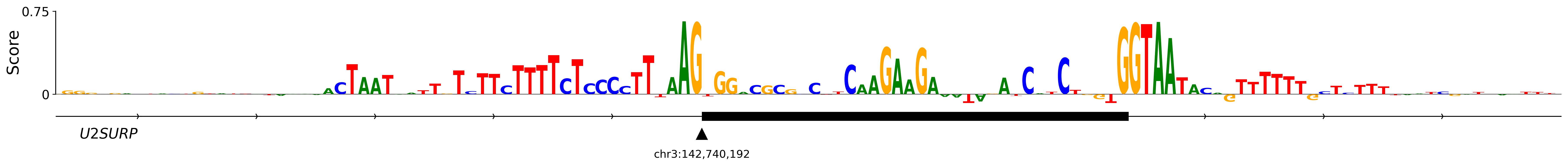
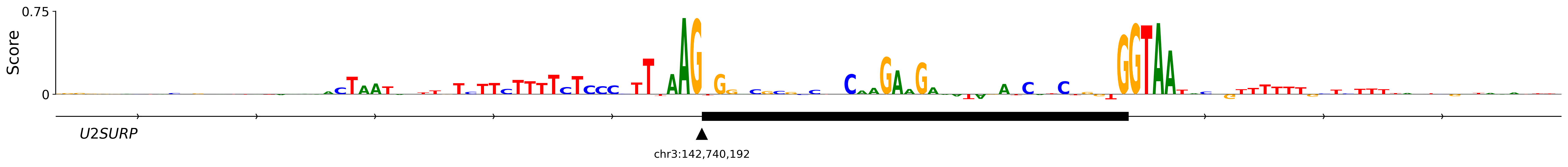
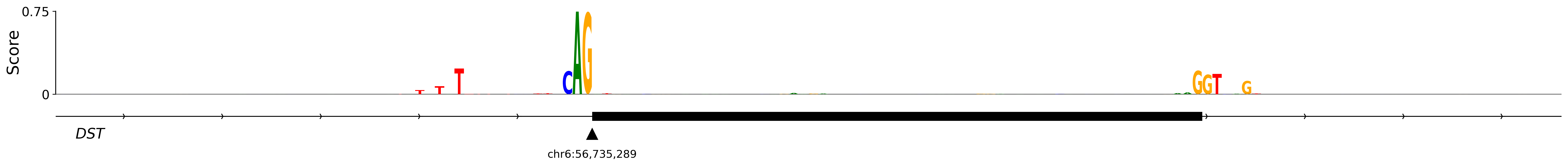
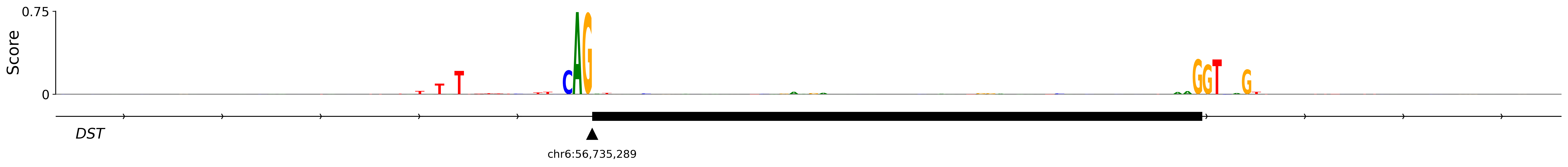
It learns similar sequence features. Accuracy alone does not show whether two models reach their predictions in the same way. In OpenSpliceAI (Chao et al., 2025), we therefore repeated an in silico mutagenesis experiment around the acceptor sites of U2SURP exon 9 and DST exon 2. At each position, we replaced the reference nucleotide with each of the other three bases and measured the average decrease in the predicted acceptor probability. The height of the reference letter in the resulting DNA sequence logo is that position’s importance score. The paired profiles below reproduce Figure 6A and make the similar patterns from SpliceAI and OpenSpliceAI easier to inspect step by step.

See which nucleotides drive an acceptor prediction

Published exampleU2SURPDST

The published examples examine the acceptor of U2SURP exon 9 and DST exon 2 together with their surrounding intronic and exonic sequence.

U2SURP exon 9

1Center the experiment on an acceptor site

U2SURP exon 9hg19 · chr3:142,740,192

upstream intronacceptorexon

Greference base

→

ACTthree substitutions

→

mean(p_ref − p_mut)importance score

SpliceAIpublished importance profile

OpenSpliceAIpublished importance profile

← Prev▶ PlayNext →↺ Restart1 / 6

ACGTacceptor position

It supports retraining across species. OpenSpliceAI can train from scratch on a new genome or initialize from a human checkpoint through transfer learning. In the paper’s mouse, zebrafish, honeybee, and Arabidopsis experiments, species-specific models outperformed direct use of the human SpliceAI model. Transfer learning converged faster and was more stable than training from random initialization in the tested settings.

It catches cryptic, disease-causing splicing. Because the variant module scores how a mutation shifts the splice landscape, OpenSpliceAI can flag the kind of cryptic splicing that underlies genetic disease — a single base change that silences a normal splice site or wakes up a dormant one. The interactive clinical walkthrough above connects those probability changes to the reported 11-bp exon extension in MYBPC3 and 54-bp cryptic exon in OPA1, while showing how closely the OpenSpliceAI and SpliceAI scores track one another.

The bigger picture

OpenSpliceAI is an argument for treating reproducibility and adaptability as part of the method. SpliceAI established a strong sequence-based architecture; OpenSpliceAI makes that architecture available as a documented PyTorch workflow for data preparation, training, calibration, transfer learning, prediction, and variant scoring. Researchers can retrain the model for another annotated genome or apply it to variants without reconstructing the training pipeline from scattered code.

That, to me, is much of what computational biology needs more of — not just better models, but open, maintained, adaptable ones. There’s plenty left to do: tissue-specific splicing, longer-range context, richer variant interpretation. But the foundation is open now, and that’s the point.

OpenSpliceAI is free and open source — the code, the trained models, and the documentation are all online.

---

Read the paper in eLife, browse the code, or work through the documentation. OpenSpliceAI was built with Alan Mao, Anqi Liu, Steven Salzberg, and Mihaela Pertea at Johns Hopkins.

References

Jaganathan, K. et al. Predicting splicing from primary sequence with deep learning. Cell (2019).doi:10.1016/j.cell.2018.12.015
Chao, K.-H., Mao, A., Salzberg, S. L., and Pertea, M. Splam: a deep-learning-based splice site predictor that improves spliced alignments. Genome Biology (2024).doi:10.1186/s13059-024-03379-4
Chao, K.-H., Mao, A., Liu, A., Salzberg, S. L., and Pertea, M. OpenSpliceAI: An efficient, modular implementation of SpliceAI enabling easy retraining on non-human species. eLife (2025).doi:10.7554/eLife.107454.3